01 - Workflow with delayflow package • delayedflow

Load package and data

library(delayedflow)
q_obs <- q_data$q_obs

Create CDCs from DFI

Now see how the DFI curve looks like:

cdc <- dfi_n(q = q_obs, n = 1:120)

head(cdc)

##   n       dfi
## 1 0 1.0000000
## 2 1 0.7898710
## 3 2 0.6637347
## 4 3 0.6014212
## 5 4 0.5483716
## 6 5 0.5194072

tail(cdc)

##       n        dfi
## 116 115 0.09210385
## 117 116 0.09210385
## 118 117 0.09210385
## 119 118 0.09210385
## 120 119 0.09210385
## 121 120 0.09210385

plot(x = 0:120, y = cdc$dfi, 
     type = "o", ylim = c(0,1),
     ylab ="DFI", xlab = "Block length N (days)",
     main = "Characteristic Delay Curve (CDC)")

Finding breakpoints

bps <- find_bps(dfi = cdc$dfi, 
               n_bp = 3,
               plotting = TRUE)

## Calculating breakpoints...Done.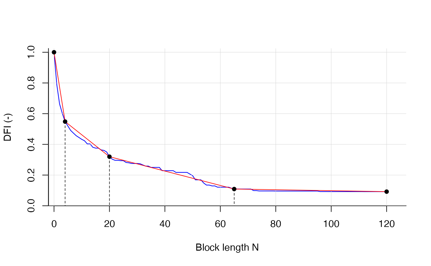

Looking at:

the breakpoint estimates, here 4, 20 and 65 days
output of the objective function
relative streamflow contributions between filter_min, the breakpoint(s) and filter_max.

bps$bps_position

## bp_1 bp_2 bp_3 
##    4   20   65

bps$bias

## [1] 0.01449936

bps$rel_contr

##   contr_1   contr_2   contr_3   contr_4 
## 0.4516284 0.2286085 0.2107172 0.1090459

Estimation of nmax

head(q_data)

##         date q_obs
## 1 2000-01-01 11.10
## 2 2000-01-02 11.20
## 3 2000-01-03 10.40
## 4 2000-01-04  9.74
## 5 2000-01-05 13.80
## 6 2000-01-06 12.80

find_nmax(q_data)

## $index_value
## [1] 0.1126447
## 
## $bp_nmax
## [1] 65

The results show that breakpoints at 65, 66 or 45 days (depending on low flow threshold) lead to a DFI value that equals the threshold.

dfi_n(q = q_data$q_obs, n = c(44:46, 64:67), add_zero = FALSE)

##    n       dfi
## 1 44 0.2173933
## 2 45 0.2173933
## 3 46 0.2173933
## 4 64 0.1144248
## 5 65 0.1090459
## 6 66 0.1090459
## 7 67 0.1090459